When I attended the Business Forecasting class at the University of Southern California, I participated to a Data Science competition in teams. The goal was to predict a year of hourly consumption of electricity of a city for an hypothetical energy supply company. More precisely, the dataset contained a time-series of four years, from 2002 to 2005, of hourly consumption, together with four different measures (average, median, minimum, maximum) of the temperature registered during that hour.
Besides forecasting hourly consumption for 2006, each team had to provide predictions of the daily peak load and the hour of the day it would have happened.
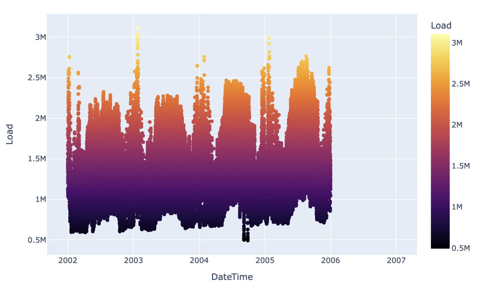
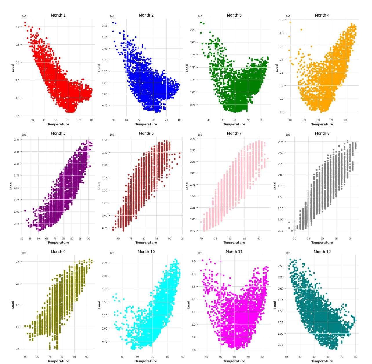
First of all, me and my team have carried out exploratory data analysis of the dataset. In particular, we wanted to investigate the different
layers of seasonality that were present in the time-series. Being the data hourly data, we hypothesised that electricity consumption could vary
on different levels:
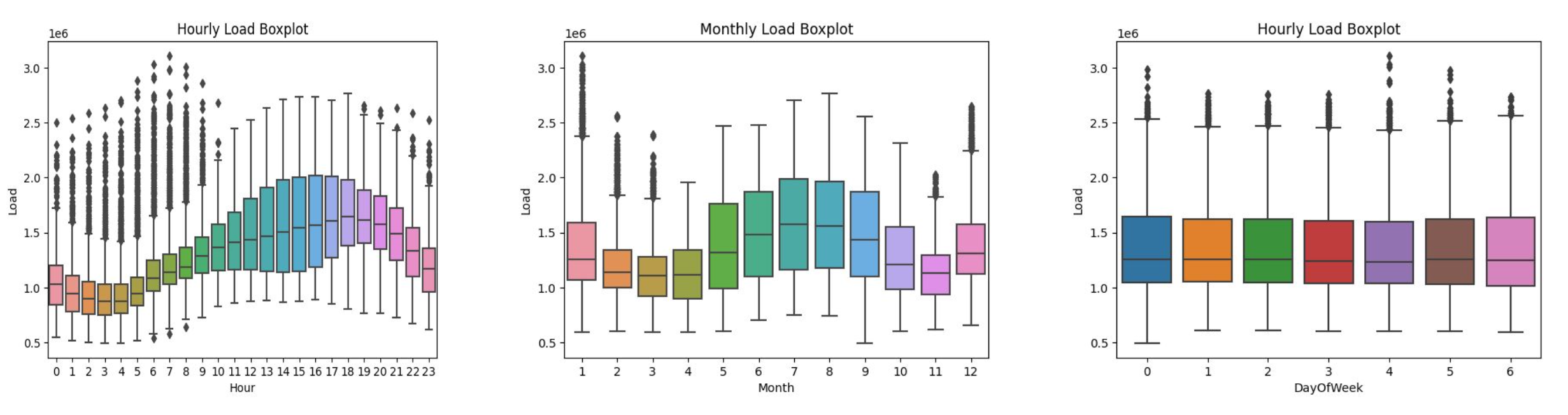
Understanding in depth this different levels of seasonality has revealed to be essential to better model the time-series. For example, we have verified that weekly seasonality seems to be not statistically significant, and that the relationship between demand of electricity and temperature is flipped between summer, when to higher temperatures corresponds higher consumption, and winter, when the opposite is true.
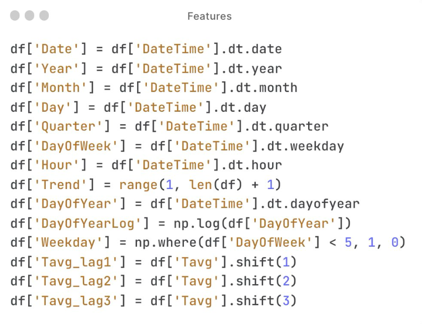
After having explored the time-series, the second phase of the project has been the construction of features that could be useful for the predictive models we would have used. First, me and my team constructed dummy variables to model the different layers of seasonality, like the hour of the day, the day, the month, the year, the quarter, and so on. Moreover, we have constructed a trend variable and lagged values of past energy consumption and past temperature.
We have divided the dataset into a train set, the years 2002-2004, and a test set, 2005. This way we could better estimate the performance of the models on new data. Then, we have trained and fine-tuned several different models, for example:
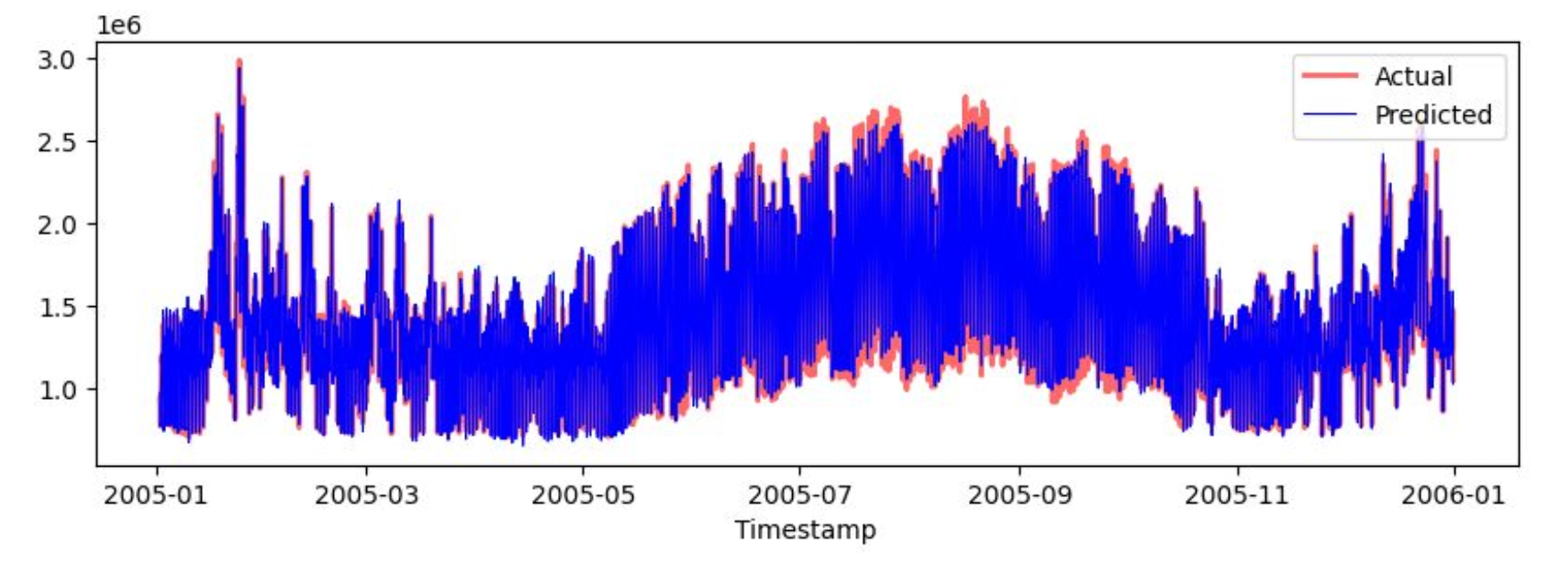
After having conducted some research, me and my team have decided to improve our XGBoost model by including some Fourier Series Components to further support the modeling of daily, weekly, and monthly seasonal effects. Moreover, we have switched to a 3-fold time-series cross-validation to better estimate the generalization capability of the model. This way, the precision of predictions increased, achieving a MAPE of 4.96%.
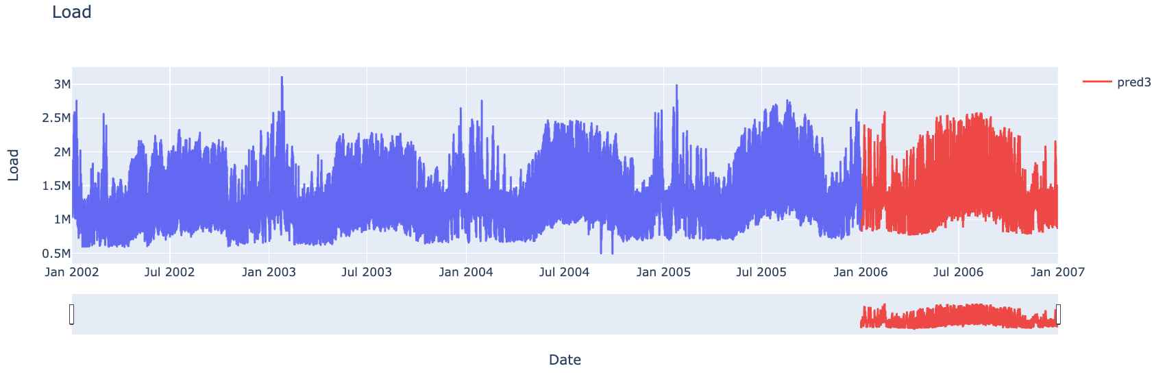
We have used our champion model to generate predictions for the year 2006. Regarding the daily peak load and its timing, we have decided to extract those predictions from the hourly predictions generated from the XGBoost model. The reason behind this choice is that, despite having trained some acceptable ad hoc models, there was the risk of delivering predictions that contradicted the forecasts of the XGBoost model. In our opinion, if the forecasts were used by a company, the indications should have been coherent, while carrying out an acceptable forecast error.